bigDM: fitting multivariate spatial models
Introduction
In previous vignettes, we show how to fit spatial Poisson mixed models for high-dimensional areal count data, how to use parallel or distributed computation strategies, and how to use the bigDM package to analyse high-dimensional spatio-temporal count data. Here, we describe how to use this package to fit order-free multivariate scalable Bayesian models to smooth mortality (or incidence) risks of several diseases simultaneously (Vicente et al., 2023).
M-models for multivariate disease mapping
Let us assume that the area of interest is divided into \(n\) contiguous small areas and data are available for \(J\) diseases. Let \(O_{ij}\) and \(E_{ij}\) denote the number of observed and expected cases respectively in the \(i\)-th small area (\(i=1, \ldots, n\)) and for the \(j\)-th disease (\(j=1, \ldots, J\)). Conditional on the relative risks \(r_{ij}\), the number of observed cases in the \(i\)-th area and the \(j\)-th disease is assumed to follow a Poisson distribution with mean \(\mu_{ij}=E_{ij} \cdot r_{ij}\), that is, \[\begin{eqnarray*} O_{ij}| r_{ij} & \sim & Poisson(\mu_{ij}=E_{ij} \cdot r_{ij}), \\ \log \mu_{ij} & = & \log E_{ij}+\log r_{ij}. \end{eqnarray*}\] Here \(E_{ij}\) is computed using indirect standardization as \(E_{ij}=\sum_{k}n_{ijk}\cdot m_{jk}\), where \(k\) is the age-group, \(n_{ijk}\) is the population at risk in area \(i\) and age-group \(k\) for the \(j\)th disease, and \(m_{jk}\) is the overall mortality (or incidence) rate of the disease \(j\) in the total area of study for the \(k\)-th age group. The log-risk is modelled as \[\begin{equation} \label{log.risk} \log r_{ij}=\alpha_j + \theta_{ij}, \end{equation}\] where \(\alpha_j\) is a disease-specific intercept and \(\theta_{ij}\) is the spatial effect of area \(i\) for the \(j\)-th disease.
Following the work by Botella-Rocamora et al. (2015), we rearrange the spatial effects into the matrix \(\Theta=\lbrace \theta_{ij} \rbrace\), for \(i=1, \ldots, n\); \(j=1, \ldots, J\) to better comprehend the dependence structure. The main advantage of the multivariate modelling is that dependence between the spatial patterns of the different diseases can be included in the model, so that latent associations between diseases can help to discover potential risk factors related to the phenomena under study. These unknown connections can be crucial to a better understanding of complex diseases such as cancer.
The potential association between the spatial patterns of the different diseases are included in the model considering the decomposition of \(\Theta\) as \[\Theta = \Phi M, \tag{1}\] where \(\Phi\) and \(M\) deal with dependency within and between diseases respectively. We refer to Equation 1 as the M-model. In the following, we briefly describe the two components of the M-model.
The matrix \(\Phi\) is a matrix of order \(n \times K\) and it is composed of stochastically independent columns that are distributed following a spatially correlated distribution. Usually, as many spatial distributions as diseases are considered, that is, \(K=J\), although \(J\) and \(K\) may be different (see Corpas-Burgos et al. (2019), for a discussion). To deal with spatial dependence, different spatial priors have been considered in the literature, most of them based on the well known intrinsic conditional autoregressive (iCAR) prior (Besag et al., 1991). See the vignette bigDM: fitting spatial models for more details.
On the other hand, \(M\) is a \(K \times J\) nonsingular but arbitrary matrix and it is responsible for inducing dependence between the different columns of \(\Theta\), i.e., for inducing corrlation between the spatial patterns of the diseases. In Equation @ref(eq:Mmodel), the cells of \(M\) act as coefficients, so they can be considered as coefficients of the log-relative risks on the underlying patterns captured in \(\Phi\) and treated as fixed effects with a normal prior distribution with mean 0 and a large (and fixed) variance. Note that, assigning \(N(0,\sigma)\) priors to the cells of \(M\) is equivalent to assigning a Wishart prior to \(M'M\), i.e., \(M'M \sim Wishart(J, \sigma^{2} \mathbf{I}_J)\). See Botella-Rocamora et al. (2015) for further details.
Once the between-diseases dependencies are incorporated into the model, the resulting prior distributions for \(\mbox{vec} \left( \Theta \right)\) with Gaussian kernel has a precision matrix given by \[\begin{equation} \Omega_{\mbox{vec}(\Theta)} = \left(M^{-1} \otimes I_n \right) \: \mbox{Blockdiag}(\Omega_{1},\ldots,\Omega_{J}) \: \left(M^{-1} \otimes I_n \right)'. \end{equation}\] Recall that this precision matrix accounts for both within and between-disease dependencies. On the one hand, the \(\Omega_{1},\ldots,\Omega_{J}\) matrices are introduced to control the within-diseases spatial variability and the between-diseases variability is captured through the matrix \(M\). Note that if \(\Omega_{1} = \ldots = \Omega_{J}= \Omega_{w}\), the covariance structure is separable and can be expressed as \(\Omega_{\mbox{vec}(\Theta)}^{-1}=\Omega_{b}^{-1} \otimes \Omega_{w}^{-1}\), where \(\Omega_{b}^{-1}=M'M\) and \(\Omega_{w}^{-1}\) are the between- and within-disease covariance matrices, respectively. This M-model based framework includes both separable and non-separable covariance structures, and can accommodate different spatial dependency structures with different within-disease covariance matrices.
Prior distributions for the disease-specific random effects
Several priors distributions are implemented in the MCAR_INLA() function to deal with spatial dependence within-diseases:
prior="intrinsic"for the M-model implementation of the intrinsic multivariate CAR latent effect.prior="Leroux"for the M-model implementation of the Leroux et al. (1999) multivariate CAR latent effect.prior="proper"for the M-model implementation of the proper multivariate CAR latent effect.prior="iid"for the M-model implementation of spatially non-structured multivariate latent effect.
As for the spatial prior distributions for univariate (single disease) models, appropriate sum-to-zero constraints must be imposed to solve identifiability problems with the disease-specific intercepts. See Vicente et al. (2023) for details about prior distributions for model hyperparameters.
Note: The M-model implementation of these models using R-INLA requires the use of at least \(J \times (J+1)/2\) hyperparameters. So, the results must be carefully checked, specially when using the LCAR or pCAR models.
Between-disease correlations and variance parameters
In addition to enlarge the effective sample size and improving smoothing by borrowing information from the different responses, one of the main advantages of multivariate disease mapping models is that they take into account correlations between the spatial patterns of the different diseases \({\rho}=(\rho_{12},\ldots,\rho_{J-1,J})^{'}\), that is, they reveal connections between diseases. In addition, it also provides the diagonal elements of the between-disease covariance matrix (\(\sigma^2_j\)), hereafter referred to as variance parameters. In the case of separable covariance structures (the kronecker product of between and within disease covariance matrices) these parameters control the amount of smoothing within diseases.
We compute the marginal posterior estimates of these parameters by sampling from the approximated joint posterior for the model hyperparameters using the inla.hyperpar.sample() function and computing kernel density estimates of the derived samples for the elements of the correlation matrix of the random effects. The results (summary statistics and posterior marginal densities) are contained in the summary.cor/summary.var and marginals.cor/marginals.var elements of the inla model.
The MCAR_INLA function
As in the CAR_INLA() and STCAR_INLA() functions, three main modelling approaches can be considered:
- the usual model with a global spatial random effect whose dependence structure is based on the whole neighbourhood graph of the areal units (
model="global"argument), - a disjoint model based on a partition of the whole spatial domain where independent spatial CAR models are simultaneously fitted in each partition (
model="partition"andk=0arguments), - a modelling approach where \(k\)-order neighbours are added to each partition to avoid border effects in the disjoint model (
model="partition"andk>0arguments).
For both the disjoint and \(k\)-order neighbour models, parallel or distributed computation strategies can be performed to speed up computations by using the future package (Bengtsson, 2021). See the vignette bigDM: parallel and distributed modelling for some examples and further details.
The data and its associated cartography file need to be specified into the MCAR_INLA() function. These are some of the most relevant arguments of this function:
carto: an object of classsforSpatialPolygonsDataFramethat must contain at least the target variable of interest specified in the argumentID.area.data: an object of classdata.framethat must contain the target variables of interest specified in the argumentsID.area,ID.disease,OandE.ID.area: name of the variable that contains the IDs of spatial areal units. The values of this variable must match those given in the carto and data variable.ID.disease: name of the variable that contains the IDs of the diseases.ID.group: name of the variable that contains the IDs of the spatial partition (grouping variable). Only required ifmodel="partition".O: name of the variable that contains the observed number of disease cases for each areal and time point.E: name of the variable that contains either the expected number of disease cases or the population at risk for each areal unit and time point.W: optional argument with the binary adjacency matrix of the spatial areal units. IfNULL(default), this object is computed from thecartoargument (two areas are considered as neighbours if they share a common border).merge.strategy: one of either"mixture"or"original"(default), that specifies the merging strategy to compute posterior marginal estimates of the linear predictor (log-risks or log-rates). SeemergeINLA()function for further details.compute.fitted.values: logical value (defaultFALSE); ifTRUEtransforms the posterior marginal distribution of the linear predictor to the exponential scale (risks or rates).
The Carto_SpainMUN object included in the bigDM package, contains the spatial polygons of the municipalities of continental Spain and simulated colorectal cancer mortality data (see the examples of the CAR_INLA function).
library(INLA)
library(bigDM)

data(Carto_SpainMUN)
head(Carto_SpainMUN)
#> Simple feature collection with 6 features and 8 fields
#> Geometry type: MULTIPOLYGON
#> Dimension:     XY
#> Bounding box:  xmin: 485318 ymin: 4727428 xmax: 543317 ymax: 4779153
#> Projected CRS: ETRS89 / UTM zone 30N
#>      ID                                    name           area    perimeter obs
#> 1 01001                        Alegria-Dulantzi 19913794 [m^2] 34372.11 [m]   2
#> 2 01002                                 Amurrio 96145595 [m^2] 63352.32 [m]  28
#> 3 01003                                 Aramaio 73338806 [m^2] 41430.46 [m]   6
#> 4 01004                              Artziniega 27506468 [m^2] 22605.22 [m]   3
#> 5 01006                                 Arminon 10559721 [m^2] 17847.35 [m]   0
#> 6 01008 Arrazua-Ubarrundia (San Martin de Ania) 57502811 [m^2] 64968.81 [m]   2
#>          exp       SMR     region                       geometry
#> 1  3.0237149 0.6614380 Pais Vasco MULTIPOLYGON (((538259 4737...
#> 2 20.8456682 1.3432047 Pais Vasco MULTIPOLYGON (((503520 4760...
#> 3  3.7527301 1.5988360 Pais Vasco MULTIPOLYGON (((533286 4759...
#> 4  3.2093191 0.9347777 Pais Vasco MULTIPOLYGON (((491260 4776...
#> 5  0.4817391 0.0000000 Pais Vasco MULTIPOLYGON (((509851 4727...
#> 6  1.9643891 1.0181282 Pais Vasco MULTIPOLYGON (((534678 4746...
In this vignette, simulated cancer mortality data for three diseases in the 7907 municipalities of mainland Spain (excluding Baleareas and Canary Islands, and the autonomous cities of Ceuta and Melilla) included in the object Data_MultiCancer will be used for illustration (modified in order to preserve the confidentiality of the original data).
data(Data_MultiCancer)
str(Data_MultiCancer)
#> 'data.frame':    23721 obs. of  5 variables:
#>  $ ID     : chr  "01001" "01002" "01003" "01004" ...
#>  $ disease: int  1 1 1 1 1 1 1 1 1 1 ...
#>  $ obs    : int  3 41 4 6 0 2 4 10 2 7 ...
#>  $ exp    : num  6.615 42.634 7.431 6.355 0.934 ...
#>  $ SMR    : num  0.454 0.962 0.538 0.944 0 ...
Note that both objects contain a common identification variable of the areal units named as ID.
Global model
We refer as Global model to the spatial multivariate model described in Equation @ref(eq:Mmodel), where the whole neighbourhood graph of the areal units is considered to define the adjacency matrix \(\textbf{W}\).
The Global model with an iCAR prior for the spatial random effects is fitted using the MCAR_INLA() function as
Global <- MCAR_INLA(carto=Carto_SpainMUN, data=Data_MultiCancer, ID.area="ID", ID.disease="disease",
O="obs", E="exp", prior="intrinsic", model="global", strategy="gaussian")
#> STEP 1: Pre-processing data
#> STEP 2: Fitting global model with INLA (this may take a while...)
summary(Global)
#> Time used:
#> Pre = 1.06, Running = 286, Post = 6.23, Total = 293
#> Fixed effects:
#> mean sd 0.025quant 0.5quant 0.975quant mode kld
#> I1 -0.139 0.006 -0.150 -0.139 -0.127 -0.139 0
#> I2 -0.049 0.006 -0.061 -0.049 -0.036 -0.049 0
#> I3 0.027 0.010 0.007 0.027 0.046 0.027 0
#>
#> Random effects:
#> Name Model
#> idx RGeneric2
#>
#> Model hyperparameters:
#> mean sd 0.025quant 0.5quant 0.975quant mode
#> Theta1 for idx -1.292 0.028 -1.348 -1.292 -1.237 -1.291
#> Theta2 for idx -1.974 0.043 -2.058 -1.974 -1.887 -1.976
#> Theta3 for idx -1.362 0.061 -1.487 -1.362 -1.240 -1.359
#> Theta4 for idx 0.118 0.010 0.098 0.118 0.138 0.118
#> Theta5 for idx 0.101 0.016 0.069 0.101 0.133 0.101
#> Theta6 for idx 0.093 0.021 0.052 0.093 0.135 0.092
#>
#> Deviance Information Criterion (DIC) ...............: 79499.30
#> Deviance Information Criterion (DIC, saturated) ....: 25184.30
#> Effective number of parameters .....................: 1721.71
#>
#> Watanabe-Akaike information criterion (WAIC) ...: 79398.24
#> Effective number of parameters .................: 1395.42
#>
#> Marginal log-Likelihood: -40195.99
#> CPO, PIT is computed
#> Posterior summaries for the linear predictor and the fitted values are computed
#> (Posterior marginals needs also 'control.compute=list(return.marginals.predictor=TRUE)')
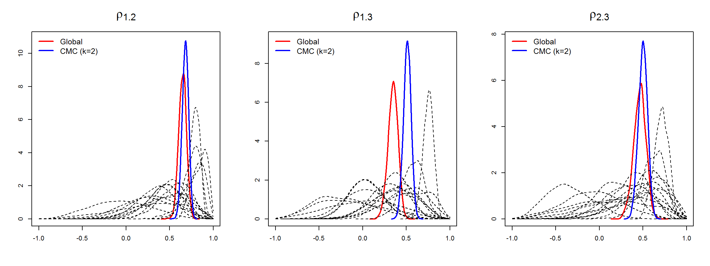
## Posterior estimates of between-disease correlations ##
Global$summary.cor
#> mean sd 0.025quant 0.5quant 0.975quant
#> rho12 0.6453091 0.03761162 0.5718745 0.6457793 0.7158483
#> rho13 0.3454653 0.05327371 0.2388130 0.3454648 0.4473405
#> rho23 0.4664424 0.05536229 0.3545904 0.4671157 0.5713110
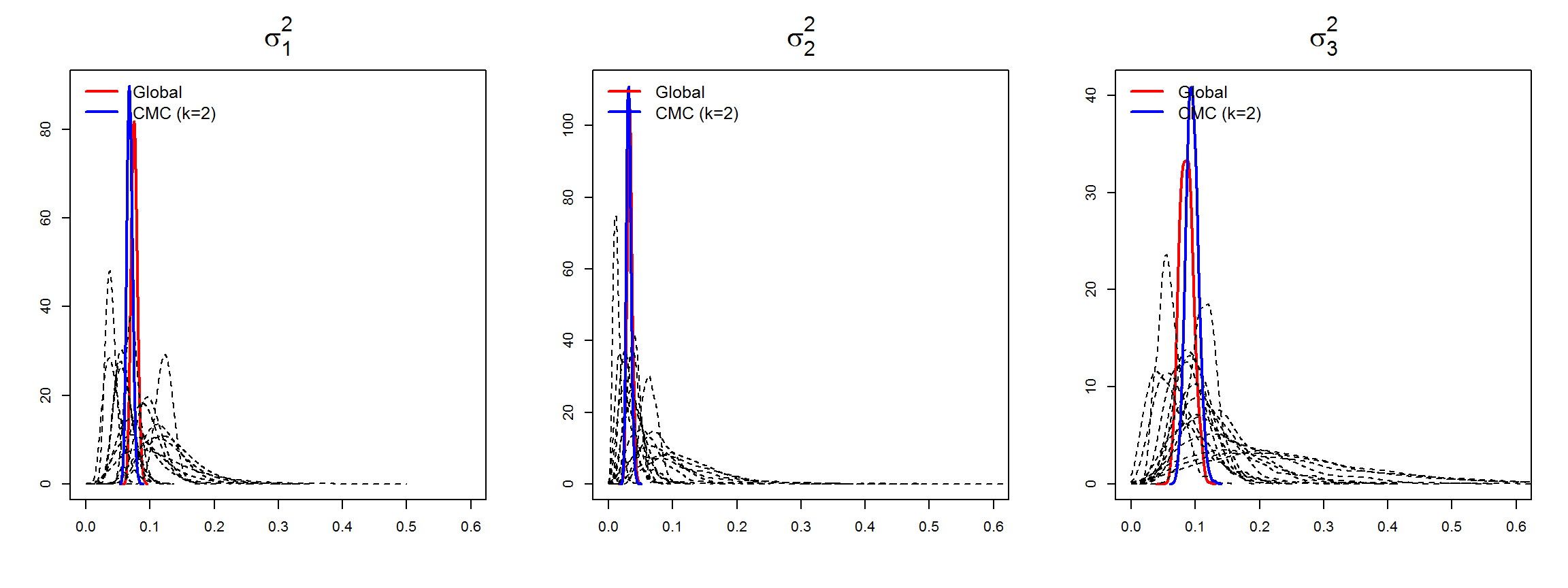
## Posterior estimates of variance parameters ##
Global$summary.var
#> mean sd 0.025quant 0.5quant 0.975quant
#> var1 0.07560148 0.004396750 0.06720687 0.07551177 0.08446323
#> var2 0.03335492 0.002931752 0.02770294 0.03333785 0.03935998
#> var3 0.08564536 0.009464110 0.06785581 0.08531868 0.10491400When the number of areas is very large, the M-model approach can be computationally very intensive. In this situation, the computational burden of these models is so high that they could be unfeasible for users with limited computing capacity. In addition, to fit a single model in the whole region could be not the best strategy as the degree of smoothing does not need to be same in the whole region. In contrast, the scalable Bayesian multivariate modelling approach described in Vicente et al. (2023) can be used to jointly smooth incidence or mortality risks of several diseases for high-dimensional areal count data. This proposal divides the spatial domain into \(D\) subregions, so that local multivariate spatial models can be fitted simultaneously (using parallel and/or distributed computation strategies) substantially reducing the computational time. In what follows, we show how to fit the Disjoint and k-order neighbourhood models extending the methodology described in Orozco-Acosta et al. (2021) for estimating spatial multivariate disease risks using the MCAR_INLA() function.
Disjoint model
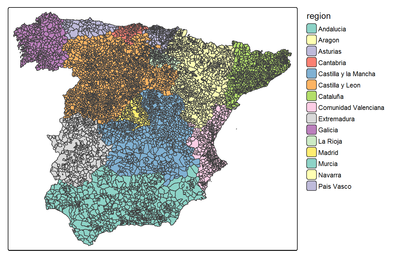
A natural way to think of partitions is to consider subregions based on administrative subdivisions of the area of interest. For our example data in Data_MultiCancer we propose to divide the data into the \(D=15\) Autonomous Regions of Spain (region variable of the Carto_SpainMUN object.
library(tmap)
tmap4 <- packageVersion("tmap") >= "3.99"

if(tmap4){
  tm_shape(Carto_SpainMUN) +
    tm_polygons(fill="region", fill.scale=tm_scale(values="brewer.set3")) +
    tm_layout(legend.frame=FALSE)
}else{
  tm_shape(Carto_SpainMUN) +
    tm_polygons(col="region") +
    tm_layout(legend.outside=TRUE)
}
In the code below, we show how to fit the Disjoint model with an iCAR prior for the spatial random effects and Gaussian approximation strategy using 4 local clusters (in parallel)
Disjoint <- MCAR_INLA(carto=Carto_SpainMUN, data=Data_MultiCancer,
                      ID.area="ID", ID.disease="disease", O="obs", E="exp", ID.group="region",
                      prior="intrinsic", model="partition", k=0, strategy="gaussian",
                      plan="cluster", workers=rep("localhost",4))
#> STEP 1: Pre-processing data
#> STEP 2: Fitting partition (k=0) model with INLA
#> + Model 1 of 15
#> + Model 2 of 15
#> + Model 3 of 15
#> + Model 4 of 15
#> + Model 5 of 15
#> + Model 6 of 15
#> + Model 7 of 15
#> + Model 8 of 15
#> + Model 9 of 15
#> + Model 10 of 15
#> + Model 11 of 15
#> + Model 12 of 15
#> + Model 13 of 15
#> + Model 14 of 15
#> + Model 15 of 15
#> STEP 3: Merging the results
summary(Disjoint)
#> Time used:
#>     Running = 195, Merging = 50.9, Total = 246, NA = NA
#> Random effects:
#>   Name     Model
#>     idx RGeneric2
#>
#> Deviance Information Criterion (DIC) ...............: 79523.29
#> Deviance Information Criterion (DIC, saturated) ....: 25217.91
#> Effective number of parameters .....................: 1979.47
#>
#> Watanabe-Akaike information criterion (WAIC) ...: 79392.49
#> Effective number of parameters .................: 1592.79
#>
#>  is computed
#> Posterior summaries for the linear predictor and the fitted values are computed
#> (Posterior marginals needs also 'control.compute=list(return.marginals.predictor=TRUE)')
* Computations are made in personal computer with a 3.41 GHz Intel Core i5-7500 processor and 32GB RAM using R-INLA stable version INLA_25.06.07.
The result is an object of class inla where the full domain log-risk is just the union of the posterior marginal estimates of each subregion, i.e., \(\log R =\left( \log R^{(1)'},\cdots,\log R^{(D)'} \right)'\). If the save.models=TRUE argument is included, a list with all the inla submodels is saved in a temporary folder, that can be used as input argument for the mergeINLA() function.
k-order neighbourhood model
As in the case of the scalable spatial and spatio-temporal models fitted with CAR_INLA() and STCAR_INLA() functions, respectively, k-order neighbourhood models can be defined to avoid the border effect of considering disjoint partitions. In this case, the entire spatial region \(\mathscr{D}\) is divided into a set of overlapping subregions and some small areas will belong to more than one of such subdivisions, i.e., \(\mathscr{D} = \bigcup_{d=1}^D \mathscr{D}_d\) but \(\mathscr{D}_i \cap \mathscr{D}_j \neq \emptyset\) for neighbouring subregions. As \(\sum_{d=1}^{D} I_{d}>n\), the final log-risk \(\log{R}=(\log{R'}_1,\ldots,\log{R'}_J)'\) with \(\log{R'}_j = (\log{R}_{1j},\ldots,\log{R}_{Ij})'\), \(j=1,\ldots,J\), is no longer the union of the posterior estimates obtained for each submodel as areas located in the borders of the spatial partition would have more than one estimated posterior distribution.
Two different merging strategies can be considered to obtain a unique posterior estimate of the linear predictor for those areas in more than one submodel:
If the
merge.strategy="original"argument is specified (default option), the posterior marginal distributions of the log-risk estimated from its original partition is used. See Orozco-Acosta et al. (2023).If the
merge.strategy="mixture"argument is specified, mixture distributions of the estimated posterior probability density functions with weights proportional to the conditional predictive ordinates (CPOs) are computed. See Orozco-Acosta et al. (2021) for further details.
In the code below, we show how to fit the 1st and 2nd-order neighbourhood model with an iCAR prior for the spatial random effects and Gaussian approximation strategy using 4 local clusters (in parallel):
order1 <- MCAR_INLA(carto=Carto_SpainMUN, data=Data_MultiCancer,
                      ID.area="ID", ID.disease="disease", O="obs", E="exp", ID.group="region",
                      prior="intrinsic", model="partition", k=1, strategy="gaussian",
                      plan="cluster", workers=rep("localhost",4))
#> STEP 1: Pre-processing data
#> STEP 2: Fitting partition (k=1) model with INLA
#> + Model 1 of 15
#> + Model 2 of 15
#> + Model 3 of 15
#> + Model 4 of 15
#> + Model 5 of 15
#> + Model 6 of 15
#> + Model 7 of 15
#> + Model 8 of 15
#> + Model 9 of 15
#> + Model 10 of 15
#> + Model 11 of 15
#> + Model 12 of 15
#> + Model 13 of 15
#> + Model 14 of 15
#> + Model 15 of 15
#> STEP 3: Merging the results
summary(order1)
#> Time used:
#>     Running = 220, Merging = 65.9, Total = 286, NA = NA
#> Deviance Information Criterion (DIC) ...............: 79468.61
#> Deviance Information Criterion (DIC, saturated) ....: 25163.24
#> Effective number of parameters .....................: 1866.37
#>
#> Watanabe-Akaike information criterion (WAIC) ...: 79360.59
#> Effective number of parameters .................: 1516.18
#>
#>  is computed
#> Posterior summaries for the linear predictor and the fitted values are computed
#> (Posterior marginals needs also 'control.compute=list(return.marginals.predictor=TRUE)')

## Posterior estimates of between-disease correlations ##
order1$summary.cor
#>            mean         sd 0.025quant  0.5quant 0.975quant
#> rho12 0.6498709 0.04126020  0.5647081 0.6509807  0.7258176
#> rho13 0.4064458 0.05238659  0.2992166 0.4071032  0.5064441
#> rho23 0.4190513 0.05944764  0.2990351 0.4194524  0.5314762

## Posterior estimates of variance parameters ##
order1$summary.var
#>            mean          sd 0.025quant   0.5quant 0.975quant
#> var1 0.06297248 0.004331878 0.05485932 0.06284425 0.07178173
#> var2 0.02725890 0.003462687 0.02111507 0.02706460 0.03456026
#> var3 0.09206563 0.009844579 0.07403273 0.09156109 0.11267122
order2 <- MCAR_INLA(carto=Carto_SpainMUN, data=Data_MultiCancer,
ID.area="ID", ID.disease="disease", O="obs", E="exp", ID.group="region",
prior="intrinsic", model="partition", k=1, strategy="gaussian",
plan="cluster", workers=rep("localhost",4))
#> STEP 1: Pre-processing data
#> STEP 2: Fitting partition (k=1) model with INLA
#> + Model 1 of 15
#> + Model 2 of 15
#> + Model 3 of 15
#> + Model 4 of 15
#> + Model 5 of 15
#> + Model 6 of 15
#> + Model 7 of 15
#> + Model 8 of 15
#> + Model 9 of 15
#> + Model 10 of 15
#> + Model 11 of 15
#> + Model 12 of 15
#> + Model 13 of 15
#> + Model 14 of 15
#> + Model 15 of 15
#> STEP 3: Merging the results
summary(order2)
#> Time used:
#> Running = 224, Merging = 66.9, Total = 291, NA = NA
#> Deviance Information Criterion (DIC) ...............: 79471.71
#> Deviance Information Criterion (DIC, saturated) ....: 25166.34
#> Effective number of parameters .....................: 1865.53
#>
#> Watanabe-Akaike information criterion (WAIC) ...: 79365.64
#> Effective number of parameters .................: 1516.64
#>
#> is computed
#> Posterior summaries for the linear predictor and the fitted values are computed
#> (Posterior marginals needs also 'control.compute=list(return.marginals.predictor=TRUE)')
## Posterior estimates of between-disease correlations ##
order2$summary.cor
#> mean sd 0.025quant 0.5quant 0.975quant
#> rho12 0.6999953 0.03347421 0.6298369 0.7016165 0.7611074
#> rho13 0.3924534 0.05182908 0.2878977 0.3928902 0.4912714
#> rho23 0.4527188 0.05741331 0.3381910 0.4538842 0.5610624
## Posterior estimates of variance parameters ##
order2$summary.var
#> mean sd 0.025quant 0.5quant 0.975quant
#> var1 0.06302142 0.004334405 0.05480051 0.06288386 0.07167173
#> var2 0.02742697 0.003112946 0.02160911 0.02732170 0.03385583
#> var3 0.09101142 0.009650894 0.07366285 0.09054036 0.11099456* Computations are made in personal computer with a 3.41 GHz Intel Core i5-7500 processor and 32GB RAM using R-INLA stable version INLA_25.06.07.
mergeINLA function
This function takes local models fitted for each subregion of the whole spatial domain and unifies them into a single inla object. It is called by the main function MCAR_INLA(), and is valid for both Disjoint and k-order neighbourhood models. In addition, approximations to model selection criteria such as the deviance information criterion (DIC) (Spiegelhalter et al., 2002) and Watanabe-Akaike information criterion (WAIC) (Watanabe, 2010) are also computed. See Vicente et al. (2023) for details on how to compute these measures for the multivariate scalable models described in this vignette.
Computation of between-disease correlation and variance parameters
Partition models provide extra information about local relationships between the diseases in the subdivisions, as they provide local estimates of model’s parameters of interest: between-disease correlations \({\rho}=(\rho_{12},\ldots,\rho_{J-1,J})^{'}\), and variance parameters \({\sigma}^2=(\sigma^2_1,\ldots,\sigma^2_J)^{'}\) (diagonal elements of the between-disease covariance matrix).
In the
mergeINLA()function, we implement an adaptation of the consensus Monte Carlo algorithm (Scott et al., 2016) to obtain global estimates of these parameters in the overall study domain from the marginal estimates of the partition models. Further details are given in Vicente et al. (2023).
Acknowledgments
This work has been supported by Project MTM2017-82553-R (AEI/FEDER, UE) and Project PID2020-113125RB-I00/MCIN/AEI/10.13039/501100011033. It has also been partially funded by the Public University of Navarra (project PJUPNA2001).