bigDM: fitting spatial models
Introduction
bigDM is a package that implements several (scalable) spatial and spatio-temporal Poisson mixed models for high-dimensional areal count data, with inference in a fully Bayesian setting using the integrated nested Laplace approximation (INLA) technique (Rue et al., 2009). This vignette focuses on how to use the bigDM package to fit the scalable spatial model’s proposals described in (Orozco-Acosta et al., 2021) using Spanish colorectal cancer mortality data.
The current stable version (0.5.7) of the package can be installed directly from CRAN
install.packages("bigDM")The development version is hosted on GitHub and can be installed as follows
# Install devtools package from CRAN repository
install.packages("devtools")

# Load devtools library
library(devtools)

# Install the R-INLA package (version 25.06.07)
install.packages("INLA", repos=c(getOption("repos"), INLA="https://inla.r-inla-download.org/R/stable"), dep=TRUE)

# In some Linux OS, it might be necessary to first install the following packages
install.packages(c("cpp11","proxy","progress","tzdb","vroom"))

# Install bigDM from GitHub repository or CRAN
install_github("spatialstatisticsupna/bigDM")
Spatial models in disease mapping
Let us assume that the spatial domain of interest is divided into \(n\) contiguous small areas labeled as \(i=1,\ldots,n\). For a given area \(i\), let \(O_i\) and \(E_i\) denote the observed and expected number of disease cases, respectively. Using these quantities, the (SMR or SIR) is defined as the ratio of observed and expected cases for the corresponding areal unit. Although its interpretation is very simple, these measures are extremely variable when analyzing rare diseases or low-populated areas, as it is the case of high-dimensional data. To cope with this situation, it is necessary to use statistical models that stabilize the risks (rates) borrowing information from neighbouring regions.
Poisson mixed models are typically used for the analysis of count data within a hierarchical Bayesian framework. Conditional to the relative risk \(r_i\), the number of observed cases in the \(i\)th area is assumed to be Poisson distributed with mean \(\mu_{i}=E_{i}r_{i}\).
That is, \[\begin{eqnarray*} \label{eq:Model_Poisson} \begin{array}{rcl} O_{i}|r_{i} & \sim & Poisson(\mu_{i}=E_{i}r_{i}), \ i=1,\ldots,n\\ \log \mu_{i} & = & \log E_{i}+\log r_{i}, \end{array} \end{eqnarray*}\] where \(\log E_{i}\) is an offset. Depending on the specification of the log-risks different models are defined.
Here we assume that \[\log{r_{i}}=\alpha+\mathbf{x_i}^{'}\beta + \xi_{i}, \tag{1}\] where \(\alpha\) is a global intercept, \(\mathbf{x_i}^{'}=(x_{i1},\ldots,x_{ip})\) is a p-vector of standardized covariates in the i-th area, \(\beta=(\beta_1,\ldots,\beta_p)\) is the p-vector of fixed effects coefficients, and \(\xi_i\) is a spatially structured random effect for which a conditional autoregressive (CAR) prior is usually assumed. The spatial correlation between CAR random effects is determined by the neighbouring structure (represented as an undirected graph) of the areal units. Let \(\textbf{W}=(w_{ij})\) be a binary \(n \times n\) adjacency matrix, whose \(ij\)th element is equal to one if areas \(j\) and \(k\) are defined as neighbours (usually if they share a common border), and it is zero otherwise.
Prior distributions
The following prior distributions are implemented in the CAR_INLA() function for the spatial random effect (specified throught the prior=... argument):
intrinsic CAR prior (iCAR)
The joint distribution of the iCAR prior (Besag et al., 1991) is defined as \[\begin{equation*} \label{eq:iCAR} \boldsymbol{\xi} \sim N(\textbf{0},\textbf{Q}^{-}_{\xi}), \quad \mbox{with} \quad \textbf{Q}_{\xi}=\tau_{\xi}(\textbf{D}_{W}-\textbf{W}) \end{equation*}\] where \(\textbf{D}_{W} = diag(w_{1+},\ldots,w_{n+})\) and \(w_{i+}=\sum_j w_{ij}\) is the \(i\)th row sum of \(\textbf{W}\), and \(\tau_{\xi}=1/\sigma^2_{\xi}\) is the precision parameter. As \(\textbf{Q}_{\xi}\textbf{1}_n=\textbf{0}\), where \(\textbf{1}_n\) is a vector of ones of length \(n\) (i.e., \(\textbf{1}_n\) is the eigenvector associated to the null eigenvalue of \(\textbf{Q}_{\xi}\)), the precision matrix of the iCAR distribution is singular and therefore, the joint distribution of \(\boldsymbol{\xi}\) is improper. If the spatial graph is fully connected (matrix \(\textbf{Q}_{\xi}\) has rank-deficiency equal to 1), a sum-to-zero constraint \(\sum_{i=1}^n \xi_i = 0\) is usually imposed to solve the identifiability issue between the spatial random effect and the intercept.
BYM prior
A convolution CAR prior (usually named as BYM prior) was also proposed by Besag et al. (1991) and combines the iCAR prior and an additional set of unstructured random effects. The model is given by \[\begin{equation*} \label{eq:BYM} \boldsymbol{\xi} = \textbf{u} + \textbf{v}, \quad \mbox{with} \quad \begin{array}{l} \textbf{u} \sim N(\textbf{0},[\tau_{u}(\textbf{D}_{W}-\textbf{W})]^{-}), \\ \textbf{v} \sim N(\textbf{0},\tau_{v}^{-1}\textbf{I}_n). \end{array} \end{equation*}\] where \(\textbf{I}_n\) is the \(n \times n\) identity matrix. The precision parameters of the spatially structured random effect (\(\tau_{u}\)) and the unstructured random effect (\(\tau_{v}\)) are not identifiable from the data , just the sum \(\xi_i=u_i + v_i\) is identifiable. Hence, similar to the iCAR prior distribution, the sum-to-zero constraint \(\sum_{i=1}^n (u_i+v_i) = 0\) must be imposed to solve identifiability problems with the intercept.
LCAR prior
Leroux et al. (1999) propose an alternative CAR prior (named as LCAR prior) to model both spatially structured and unstructured variation in a single set of random effects. It is given by \[\begin{equation*} \label{eq:LCAR} \boldsymbol{\xi} \sim N(\textbf{0},\textbf{Q}^{-1}_{\xi}), \quad \mbox{with} \quad \textbf{Q}_{\xi}=\tau_{\xi}[\lambda_{\xi}(\textbf{D}_W-{\textbf{W}})+(1-\lambda_{\xi})\textbf{I}_n] \end{equation*}\] where \(\tau_{\xi}\) is the precision parameter and \(\lambda_{\xi} \in [0,1]\) is a spatial smoothing parameter. Even the precision matrix \(\textbf{Q}_{\xi}\) is of full rank whenever \(0 \leq \lambda_{\xi} < 1\), a confounding problem still remains and consequently, a sum-to-zero constraint \(\sum_{i=1}^n \xi_i = 0\) has to be considered (see Goicoa et al. (2018)).
BYM2 prior
In Riebler et al. (2016) a modification of the Dean et al. (2001) model was proposed which addresses both the identifiability and scaling issue of the BYM model, hereafter BYM2 model. Here, the spatial random effect is reparameterized as \[\begin{equation} \label{eq:BYM2} \boldsymbol{\xi} = \frac{1}{\sqrt{\tau_{\xi}}}(\sqrt{\lambda_{\xi}}\textbf{u}_{\star} + \sqrt{1-\lambda_{\xi}}\textbf{v}), \end{equation}\] where \(\textbf{u}_{\star}\) is the scaled intrinsic CAR model with generalized variance equal to one and \(\textbf{v}\) is the vector of unstructured random effects. The variance of is expressed as a weighted average of the covariance matrices of the structured and unstructured spatial components (unlike the LCAR model which considers a weighted combination of the precision matrices), i.e., \[\begin{equation*} \mbox{Var}(\boldsymbol{\xi}|\tau_{\xi})=\frac{1}{\tau_{\xi}}(\lambda_{\xi}\textbf{R}_{\star}^{-} + (1-\lambda_{\xi})\textbf{I}_n), \end{equation*}\] where \(\textbf{R}_{\star}^{-}\) indicates the generalised inverse of the scaled spatial precision matrix (Sørbye & Rue, 2014). As in the previous models, a sum-to-zero constraint \(\sum_{i=1}^n \xi_i =0\) must be imposed to avoid identifiability problems.
By default (PCpriors=FALSE argument), improper uniform prior distributions on the positive real line are considered for the standard deviations, i.e., \(\sigma_{\xi} = 1/\sqrt{\tau_{\xi}} \sim U(0,\infty)\). In addition, a standard uniform distribution is given to the spatial smoothing parameter \(\lambda_{\xi}\) when fitting the LCAR or BYM2 model for the spatial random effect. See Ugarte et al. (2016) for details about how to implement these hyperprior distributions in R-INLA.
If setting PCpriors=TRUE argument, then penalised complexity (PC) priors (Simpson et al., 2017) are used for the precision parameter of the spatial random effect \(\boldsymbol{\xi}\). This option only works if iCAR (prior="intrinsic" argument) or BYM2 (prior="BYM2" argument) spatial prior distributions are selected. In both cases, the default values in R-INLA \((U,\alpha)=(1,0.1)\) are considered for the standard deviation of the random effect, which means that \(P(\sigma_{\xi}>1)=0.1\). If the BYM2 model is selected, the values \((U,\alpha)=(0.5,0.5)\) are also given to the spatial smoothing parameter \(\lambda_{\xi}\), that is, \(P(\lambda_{\xi}>0.5)=0.5\).
INLA approximation strategy
The following approximation strategies are implemented in R-INLA: Gaussian (strategy="gaussian"), simplified Laplace (strategy="simplified.laplace") or full Laplace (strategy="laplace"). The Gaussian approximation is the fastest option and often gives reasonable results, but it may be inaccurate. The full Laplace approximation is very accurate, but it can be computationally expensive. The simplified Laplace approximation (default option in CAR_INLA() function) offers a tradeoff between accuracy and computing time. See Rue et al. (2009) for details about the approximation strategies in INLA.
Initial step: input argument for the CAR_INLA function
The input argument of the CAR_INLA() function must be an object of class sf or SpatialPolygonsDataFrame that contains the data of analysis and its associated cartography file. Note that bigDM includes the Carto_SpainMUN sf (simple feature) object containing the polygons of Spanish municipalities and simulated colorectal cancer mortality data (modified in order to preserve the confidentiality of the original data).
library(INLA)
library(bigDM)

head(Carto_SpainMUN)
#> Simple feature collection with 6 features and 8 fields
#> Geometry type: MULTIPOLYGON
#> Dimension:     XY
#> Bounding box:  xmin: 485318 ymin: 4727428 xmax: 543317 ymax: 4779153
#> Projected CRS: ETRS89 / UTM zone 30N
#>      ID                                    name           area    perimeter obs
#> 1 01001                        Alegria-Dulantzi 19913794 [m^2] 34372.11 [m]   2
#> 2 01002                                 Amurrio 96145595 [m^2] 63352.32 [m]  28
#> 3 01003                                 Aramaio 73338806 [m^2] 41430.46 [m]   6
#> 4 01004                              Artziniega 27506468 [m^2] 22605.22 [m]   3
#> 5 01006                                 Arminon 10559721 [m^2] 17847.35 [m]   0
#> 6 01008 Arrazua-Ubarrundia (San Martin de Ania) 57502811 [m^2] 64968.81 [m]   2
#>          exp       SMR     region                       geometry
#> 1  3.0237149 0.6614380 Pais Vasco MULTIPOLYGON (((538259 4737...
#> 2 20.8456682 1.3432047 Pais Vasco MULTIPOLYGON (((503520 4760...
#> 3  3.7527301 1.5988360 Pais Vasco MULTIPOLYGON (((533286 4759...
#> 4  3.2093191 0.9347777 Pais Vasco MULTIPOLYGON (((491260 4776...
#> 5  0.4817391 0.0000000 Pais Vasco MULTIPOLYGON (((509851 4727...
#> 6  1.9643891 1.0181282 Pais Vasco MULTIPOLYGON (((534678 4746...
In what follows, we describe how to create this object in R from a cartography shapefile (.shp) format and data file (.csv) containing the data of analysis:
- Read the shapefile of Spanish municipalities as an object of class
sf
library(sf)

## Download and extract the zip file containing the shapefile ##
temp.file <- tempfile()
filename <- paste(temp.file,"zip",sep=".")
curl::curl_download(
  url = "https://emi-sstcdapp.unavarra.es/bigDM/inst/shape/Carto_SpainMUN.zip",
  destfile = "Carto_SpainMUN.zip",
  handle = curl::new_handle(ssl_verifypeer=0, ssl_verifyhost=0)
)
unzip("Carto_SpainMUN.zip",exdir=temp.file)

## Read the shapefile as a 'sf' object ##
carto_sf <- st_read(temp.file)
#> Reading layer `Carto_SpainMUN' from data source
#>   `C:\Users\aritz.adin.DYC\AppData\Local\Temp\Rtmp4kiikH\file390464a14a66'
#>   using driver `ESRI Shapefile'
#> Simple feature collection with 7907 features and 10 fields
#> Geometry type: MULTIPOLYGON
#> Dimension:     XY
#> Bounding box:  xmin: -13952 ymin: 3987408 xmax: 1021167 ymax: 4859444
#> Projected CRS: ETRS89 / UTM zone 30N- If necessary, read the csv file with the simulated colorectal cancer mortality data and merge with the cartography file. Note that both files must contain a common identifier variable for the areas (polygons).
library(readr)

curl::curl_download(
  url = "https://emi-sstcdapp.unavarra.es/bigDM/inst/csv/data.csv",
  destfile = "data.csv",
  handle = curl::new_handle(ssl_verifypeer = 0, ssl_verifyhost = 0)
)

data <- read_csv("data.csv")
#> Rows: 7907 Columns: 3
#> -- Column specification --------------------------------------------------------
#> Delimiter: ","
#> chr (1): ID
#> dbl (2): obs, exp
#>
#> i Use `spec()` to retrieve the full column specification for this data.
#> i Specify the column types or set `show_col_types = FALSE` to quiet this message.
carto <- merge(carto_sf, data, by="ID")

head(carto)
#> Simple feature collection with 6 features and 12 fields
#> Geometry type: MULTIPOLYGON
#> Dimension:     XY
#> Bounding box:  xmin: 485318 ymin: 4727428 xmax: 543317 ymax: 4779153
#> Projected CRS: ETRS89 / UTM zone 30N
#>      ID                                    name     lat    long     area
#> 1 01001                        Alegria-Dulantzi 4742974 4742974 19913794
#> 2 01002                                 Amurrio 4765886 4765886 96145595
#> 3 01003                                 Aramaio 4766225 4766225 73338806
#> 4 01004                              Artziniega 4775453 4775453 27506468
#> 5 01006                                 Arminon 4729884 4729884 10559721
#> 6 01008 Arrazua-Ubarrundia (San Martin de Ania) 4752714 4752714 57502811
#>   perimeter obs.x      exp.x       SMR     region obs.y      exp.y
#> 1  34372.11     2  3.0237149 0.6614380 Pais Vasco     2  3.0237149
#> 2  63352.32    28 20.8456682 1.3432047 Pais Vasco    28 20.8456682
#> 3  41430.46     6  3.7527301 1.5988360 Pais Vasco     6  3.7527301
#> 4  22605.22     3  3.2093191 0.9347777 Pais Vasco     3  3.2093191
#> 5  17847.35     0  0.4817391 0.0000000 Pais Vasco     0  0.4817391
#> 6  64968.81     2  1.9643891 1.0181282 Pais Vasco     2  1.9643891
#>                         geometry
#> 1 MULTIPOLYGON (((538259 4737...
#> 2 MULTIPOLYGON (((503520 4760...
#> 3 MULTIPOLYGON (((533286 4759...
#> 4 MULTIPOLYGON (((491260 4776...
#> 5 MULTIPOLYGON (((509851 4727...
#> 6 MULTIPOLYGON (((534678 4746...
Global model
We denote as Global model to the spatial model described in Equation 1, where the whole neighbourhood graph of the areal units is considered to define the adjacency matrix \(\textbf{W}\).
The Global model is fitted using the CAR_INLA() function as
## Not run:
Global <- CAR_INLA(carto=Carto_SpainMUN, ID.area="ID", O="obs", E="exp", model="global")
where ID is a character vector of geographic identifiers of the Spanish municipalities, while obs and exp are the variables with the observed and expected number of colorectal cancer mortality cases in each municipality, respectively.
By default, the LCAR prior distribution is considered for the spatial random effect \(\boldsymbol{\xi}\), and the simplified Laplace approximation strategy is used to fit the model (arguments prior="Leroux" and strategy="simplified.laplace, respectively).
Disjoint model
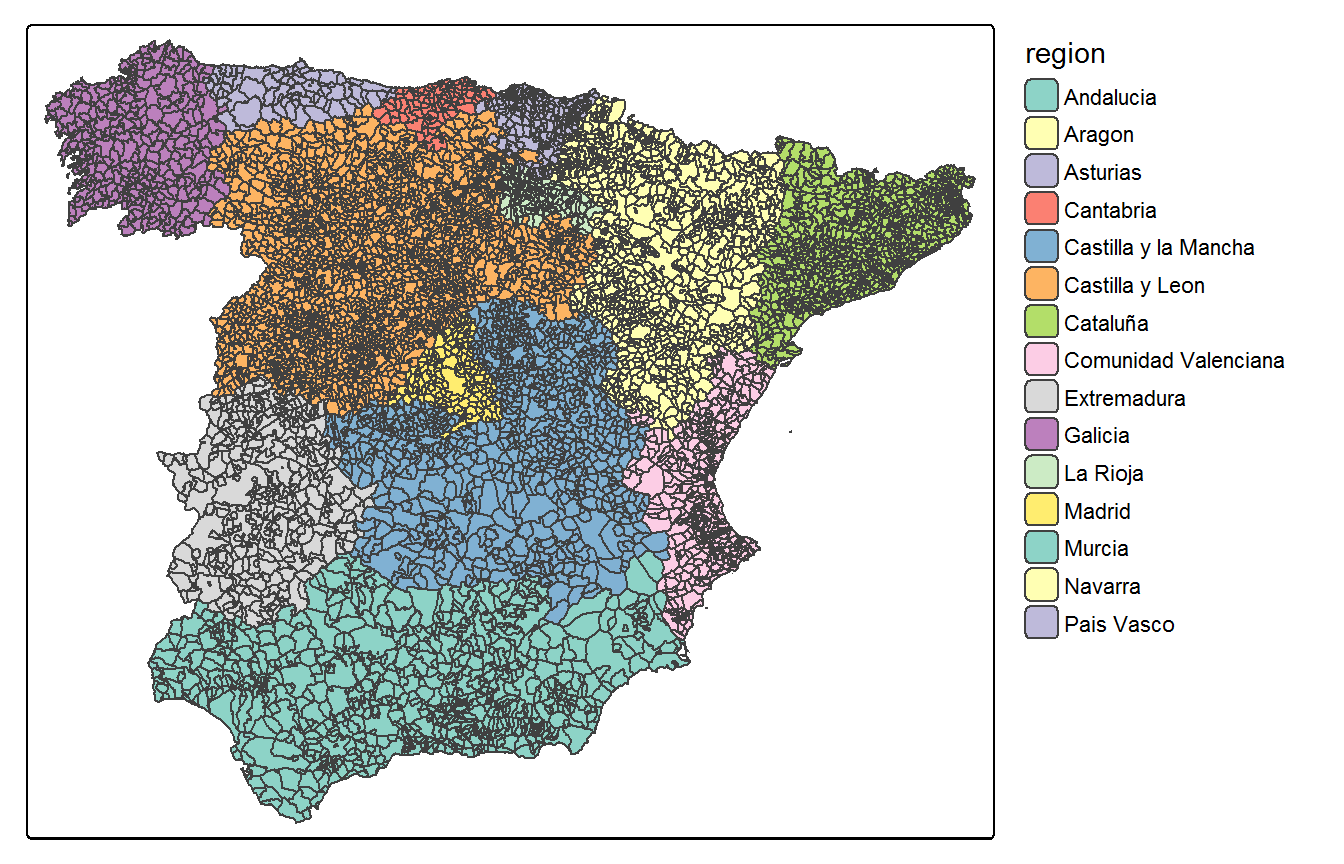
The key idea of the Disjoint model is to define a partition of the whole spatial domain \(\mathscr{D}\) into \(D\) subregions, that is \(\mathscr{D} = \bigcup_{d=1}^D \mathscr{D}_d\) where \(\mathscr{D}_i \cap \mathscr{D}_j = \emptyset\) for all \(i \neq j\). In our disease mapping context, this means that each geographical unit belongs to a single subregion. A natural choice for this partition could be the administrative subdivisions of the area of interest (such as for example, provinces or states). For our example data in Carto_SpainMUN the \(D=15\) Autonomous Regions of Spain are used as a partition of the \(n=7907\) municipalites (region variable of the sf object).
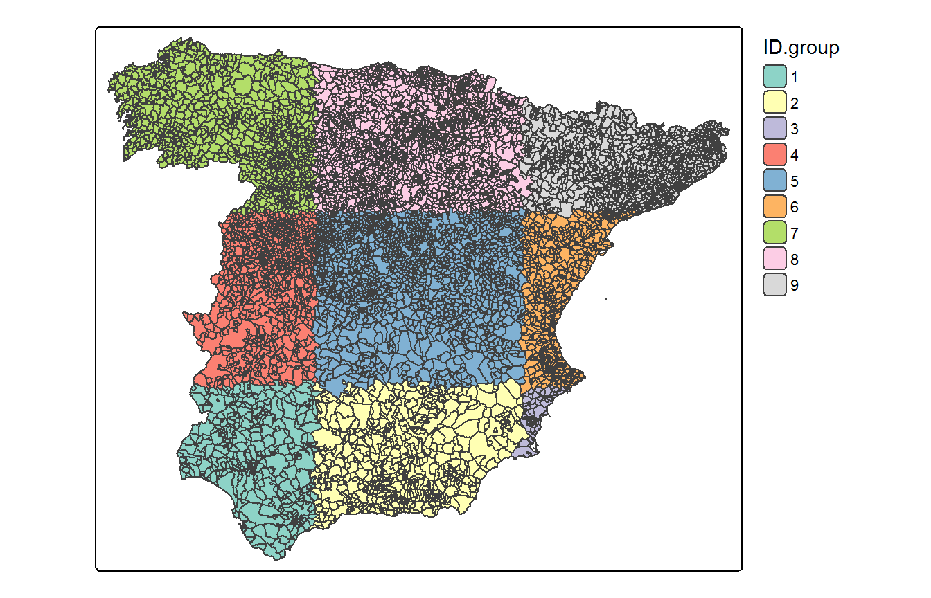
If the user has no idea on how to define this initial partition, the random_partition() function can be used to define a regular grid over the associated cartography with a certain number of rows and columns. For example, let us define a random partition for the Spanish municipalities based on a 3x3 regular grid
carto.new <- random_partition(carto=Carto_SpainMUN, rows=3, columns=3, max.size=NULL)The result is an object of class sf with the original data and a grouping variable named ID.group. We can use this variable to plot the spatial partition using the tmap library as
library(tmap)
tmap4 <- packageVersion("tmap") >= "3.99"

if(tmap4){
  tm_shape(carto.new) +
    tm_polygons(fill="ID.group", fill.scale=tm_scale(values="brewer.set3")) +
    tm_layout(legend.frame=FALSE)
}else{
  tm_shape(carto.new) +
    tm_polygons(col="ID.group") +
    tm_layout(legend.outside=TRUE)
}
Once the partition variable is defined, the Disjoint model is fitted using the CAR_INLA() function as
Disjoint <- CAR_INLA(carto=Carto_SpainMUN, ID.area="ID", ID.group="region", O="obs", E="exp",
                     model="partition", k=0, strategy="gaussian", save.models=TRUE)
#> STEP 1: Pre-processing data
#> STEP 2: Fitting partition (k=0) model with INLA
#> + Model 1 of 15
#> + Model 2 of 15
#> + Model 3 of 15
#> + Model 4 of 15
#> + Model 5 of 15
#> + Model 6 of 15
#> + Model 7 of 15
#> + Model 8 of 15
#> + Model 9 of 15
#> + Model 10 of 15
#> + Model 11 of 15
#> + Model 12 of 15
#> + Model 13 of 15
#> + Model 14 of 15
#> + Model 15 of 15
#> + Saving all the inla submodels in '/temp/' folder
#> STEP 3: Merging the results

summary(Disjoint)
#> Time used:
#>     Running = 55.1, Merging = 21.2, Total = 76.3, NA = NA
#> Random effects:
#>   Name     Model
#>     ID.area Generic1 model
#>
#> Deviance Information Criterion (DIC) ...............: 27454.49
#> Deviance Information Criterion (DIC, saturated) ....: 8391.04
#> Effective number of parameters .....................: 403.25
#>
#> Watanabe-Akaike information criterion (WAIC) ...: 27435.61
#> Effective number of parameters .................: 341.61
#>
#>  is computed
#> Posterior summaries for the linear predictor and the fitted values are computed
#> (Posterior marginals needs also 'control.compute=list(return.marginals.predictor=TRUE)')
* Computations are made in personal computer with a 3.41 GHz Intel Core i5-7500 processor and 32GB RAM using R-INLA stable version INLA_25.06.07.
The result is an object of class inla where the log-risks \(\log{r_i}\) are just the union of the posterior marginal estimates of each submodel. If the save.models=TRUE argument is included, a list with all the inla submodels is saved in temporary folder, which can be used as input argument for the mergeINLA() function.
k-order neighbourhood models
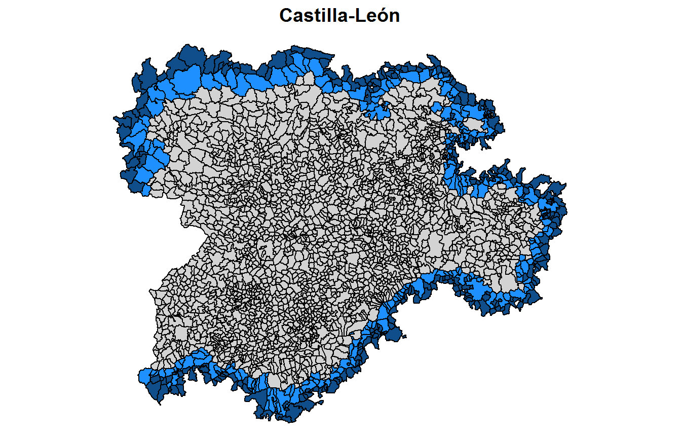
To avoid border effects in the disease mapping estimates when fitting the Disjoint model, we also propose a second modeling approach where \(k\)-order neighbours are added to each subregion of the spatial domain. Doing so, \(\mathscr{D}\) is now divided into overlapping set of regions, that is, \(\mathscr{D} = \bigcup_{d=1}^D \mathscr{D}_d\) but \(\mathscr{D}_i \cap \mathscr{D}_j \neq \emptyset\) for neighbouring subregions. This implies that, for some areal units, multiple risk estimates will be obtained from the different local submodels and consequently, their posterior estimates must be properly combined to obtain a single posterior distribution for each area. Originally, Orozco et al. (2021) propose to compute mixture distributions of the estimated posterior probability functions with weights proportional to the conditional predictive ordinates (CPO). However, in Orozco et al. (2023) we also investigate the strategy of using the posterior marginal estimates of the areal-unit corresponding to the original submodel, which performs better in terms of risk estimation accuracy and computational time. Further details are given below.
The k-order neighbourhood model is fitted using the CAR_INLA() function as
## 1st order neighbourhood model ##
order1 <- CAR_INLA(carto=Carto_SpainMUN, ID.area="ID", ID.group="region", O="obs", E="exp",
                   model="partition", k=1, strategy="gaussian", save.models=TRUE)
#> STEP 1: Pre-processing data
#> STEP 2: Fitting partition (k=1) model with INLA
#> + Model 1 of 15
#> + Model 2 of 15
#> + Model 3 of 15
#> + Model 4 of 15
#> + Model 5 of 15
#> + Model 6 of 15
#> + Model 7 of 15
#> + Model 8 of 15
#> + Model 9 of 15
#> + Model 10 of 15
#> + Model 11 of 15
#> + Model 12 of 15
#> + Model 13 of 15
#> + Model 14 of 15
#> + Model 15 of 15
#> + Saving all the inla submodels in '/temp/' folder
#> STEP 3: Merging the results
summary(order1)
#> Time used:
#>     Running = 60.3, Merging = 29.9, Total = 90.1, NA = NA
#> Deviance Information Criterion (DIC) ...............: 27440.41
#> Deviance Information Criterion (DIC, saturated) ....: 8376.97
#> Effective number of parameters .....................: 399.31
#>
#> Watanabe-Akaike information criterion (WAIC) ...: 27425.04
#> Effective number of parameters .................: 339.73
#>
#>  is computed
#> Posterior summaries for the linear predictor and the fitted values are computed
#> (Posterior marginals needs also 'control.compute=list(return.marginals.predictor=TRUE)')

## 2nd order neighbourhood model ##
order2 <- CAR_INLA(carto=Carto_SpainMUN, ID.area="ID", ID.group="region", O="obs", E="exp",
                   model="partition", k=2, strategy="gaussian", save.models=TRUE)
#> STEP 1: Pre-processing data
#> STEP 2: Fitting partition (k=2) model with INLA
#> + Model 1 of 15
#> + Model 2 of 15
#> + Model 3 of 15
#> + Model 4 of 15
#> + Model 5 of 15
#> + Model 6 of 15
#> + Model 7 of 15
#> + Model 8 of 15
#> + Model 9 of 15
#> + Model 10 of 15
#> + Model 11 of 15
#> + Model 12 of 15
#> + Model 13 of 15
#> + Model 14 of 15
#> + Model 15 of 15
#> + Saving all the inla submodels in '/temp/' folder
#> STEP 3: Merging the results
summary(order2)
#> Time used:
#>     Running = 70.6, Merging = 30.9, Total = 101, NA = NA
#> Deviance Information Criterion (DIC) ...............: 27448.45
#> Deviance Information Criterion (DIC, saturated) ....: 8385.00
#> Effective number of parameters .....................: 375.53
#>
#> Watanabe-Akaike information criterion (WAIC) ...: 27438.38
#> Effective number of parameters .................: 323.40
#>
#>  is computed
#> Posterior summaries for the linear predictor and the fitted values are computed
#> (Posterior marginals needs also 'control.compute=list(return.marginals.predictor=TRUE)')
* Computations are made in personal computer with a 3.41 GHz Intel Core i5-7500 processor and 32GB RAM using R-INLA stable version INLA_25.06.07.
Internally, the divide_carto() function is called to compute the overlapping set of regions \(\{\mathscr{D}_1, \ldots, \mathscr{D}_D\}\) according to some grouping variable (the "region" variable in the previous example). By default, a disjoint partition (k=0 argument) is defined by this function. In Figure @ref(fig:disjointPartition), the disjoint partition for the Spanish municipalities based on the \(D=15\) autonomous regions is plotted.
The neighbourhood order to add polygons at the border of the spatial subdomains is controlled by the k argument.
## disjoint partition ##
carto.k0 <- divide_carto(carto=Carto_SpainMUN, ID.group="region", k=0)

## 1st order partition ##
carto.k1 <- divide_carto(carto=Carto_SpainMUN, ID.group="region", k=1)

## 2nd order partition ##
carto.k2 <- divide_carto(carto=Carto_SpainMUN, ID.group="region", k=2)
where the output of the divide_carto() function is a list of sf objects of length \(D\) with the spatial polygons for each subdomain.
mergeINLA function
This function takes local models fitted for each subregion of the whole spatial domain and unifies them into a single inla object. It is called by the main function CAR_INLA(), and is valid for both Disjoint and k-order neighbourhood models. In addition, approximations to model selection criteria such as the deviance information criterion (DIC) (Spiegelhalter et al., 2002) and Watanabe-Akaike information criterion (WAIC) (Watanabe, 2010) are also computed. See Orozco et al. (2021) for details on how to compute these measures for the scalable model proposals that are available in the bigDM package.
Merging strategy
If the k-order neighbourhood model is fitted, note that the final log-risk surface \(\log{\textbf{r}} = (\log{r_1},\ldots,\log{r_n})^{'}\) is no longer the union of the posterior estimates obtained from each submodel. To obtain a unique posterior distribution of \(\log{r_i}\) for each areal unit \(i\), two merging strategies could be considered.
- If the
merge.strategy="original"argument is specified (default option), the posterior marginal estimate ot the areal-unit corresponding to the original submodel is selected. - If the
merge.strategy="mixture"argument is specified, mixture distributions of the estimated posterior probability density functions with weights proportional to the conditional predictive ordinates (CPO) are computed. See Orozco et al. (2021) for further details.
- If the
In what follows, we show how to use the mergeINLA() function to reproduce the results obtained with the main CAR_INLA() function using the previously saved models for each spatial subdomain. The corresponding .Rdata objects have been renamed as INLAsubmodels_Disjoint.Rdata, INLAsubmodels_order1.Rdata and INLAsubmodels_order2.Rdata.
## Disjoint model ##
load("temp/INLAsubmodels_Disjoint.Rdata")

Disjoint <- mergeINLA(inla.models=inla.models, k=0, n.sample=1000,
                      compute.DIC=TRUE, compute.fitted.values=TRUE)

summary(Disjoint)
#> Time used:
#>     Running = 55.1, Merging = 46.3, Total = 101, NA = NA
#> Random effects:
#>   Name     Model
#>     ID.area Generic1 model
#>
#> Deviance Information Criterion (DIC) ...............: 27453.33
#> Deviance Information Criterion (DIC, saturated) ....: 8389.89
#> Effective number of parameters .....................: 403.10
#>
#> Watanabe-Akaike information criterion (WAIC) ...: 27435.62
#> Effective number of parameters .................: 341.66
#>
#>  is computed
#> Posterior summaries for the linear predictor and the fitted values are computed
#> (Posterior marginals needs also 'control.compute=list(return.marginals.predictor=TRUE)')

## 1st order neighbourhood model ##
load("temp/INLAsubmodels_order1.Rdata")

order1 <- mergeINLA(inla.models=inla.models, k=1, n.sample=1000,
                    compute.DIC=TRUE, compute.fitted.values=TRUE)

summary(order1)
#> Time used:
#>     Running = 60.3, Merging = 53.2, Total = 113, NA = NA
#> Deviance Information Criterion (DIC) ...............: 27440.32
#> Deviance Information Criterion (DIC, saturated) ....: 8376.88
#> Effective number of parameters .....................: 399.69
#>
#> Watanabe-Akaike information criterion (WAIC) ...: 27421.47
#> Effective number of parameters .................: 338.20
#>
#>  is computed
#> Posterior summaries for the linear predictor and the fitted values are computed
#> (Posterior marginals needs also 'control.compute=list(return.marginals.predictor=TRUE)')

## 2nd order neighbourhood model ##
load("temp/INLAsubmodels_order2.Rdata")

order2 <- mergeINLA(inla.models=inla.models, k=2, n.sample=1000,
                    compute.DIC=TRUE, compute.fitted.values=TRUE)

summary(order2)
#> Time used:
#>     Running = 70.6, Merging = 52.9, Total = 124, NA = NA
#> Deviance Information Criterion (DIC) ...............: 27444.79
#> Deviance Information Criterion (DIC, saturated) ....: 8381.35
#> Effective number of parameters .....................: 374.03
#>
#> Watanabe-Akaike information criterion (WAIC) ...: 27433.03
#> Effective number of parameters .................: 321.02
#>
#>  is computed
#> Posterior summaries for the linear predictor and the fitted values are computed
#> (Posterior marginals needs also 'control.compute=list(return.marginals.predictor=TRUE)')
* Computations are made in personal computer with a 3.41 GHz Intel Core i5-7500 processor and 32GB RAM using R-INLA stable version INLA_25.06.07.
Acknowledgments
This work has been supported by Project MTM2017-82553-R (AEI/FEDER, UE) and Project PID2020-113125RB-I00/MCIN/AEI/10.13039/501100011033. It has also been partially funded by the Public University of Navarra (project PJUPNA2001).