bigDM: fitting spatio-temporal models
Introduction
In previous vignettes, we show how to fit spatial Poisson mixed models for high-dimensional areal count data and how to use parallel or distributed computation strategies using the bigDM package. Here, we describe how to use this package to fit spatio-temporal models with conditional autoregressive (CAR) priors for space and random walk (RW) priors for time including space-time interactions (Knorr-Held, 2000; Ugarte et al., 2014) by extending the scalable model’s proposals described in Orozco-Acosta et al. (2021) to deal with massive spatio-temporal data (Orozco-Acosta et al., 2023).
Spatio-temporal models in disease mapping
Let us assume that the region under study is divided into \(n\) contiguous small areas labeled as \(i=1,\ldots,n\) and data are available for consecutive time periods labeled as \(t=1,\ldots,T\). For a given area \(i\) and time period \(t\),
- \(O_{it}\) denotes the number of observed cases for area \(i\) and time \(t\)
- \(E_{it}\) denotes the number of expected cases for area \(i\) and time \(t\)
- \(r_{it}\) is the relative risk of mortality (incidence)
To compute the number of expected cases \(E_{it}\), both direct and indirect standardization procedures can be performed (Ugarte, 2009), usually considering age and/or sex as standardization variables. Using the indirect standardization method, the number of expected cases for area \(i\) and time \(t\) is defined as
\[E_{it}=\sum_{j=1}^{J}N_{it}\frac{O_j}{N_j} \ \ \mbox{for} \ \ i=1,\ldots,n; \ \ t=1,\ldots,T,\] where \(O_j=\sum_{i=1}^{n}\sum_{t=1}^{T}O_{itj}\) and \(N_j=\sum_{i=1}^{n}\sum_{t=1}^{T}N_{itj}\) are the number of observed cases and the population at risk in the \(j^{th}\) age-group, respectively. Then, the standardized mortality/incidence ratio (SMR or SIR) is defined as the number of observed cases divided by the number of expected cases. Although its interpretation is very simple, these measures are extremely variable when analyzing rare diseases or very low-populated areas, as it is the case of high-dimensional data. This makes it necessary the use of statistical models to smooth risks borrowing information from neighbouring regions and time periods.
Poisson mixed models are typically used for the analysis of count data within a hierarchical Bayesian framework. Conditional to the relative risk \(r_{it}\), the number of observed cases in the \(i\)th area and time period \(t\) is assumed to be Poisson distributed with mean \(\mu_{it} = E_{it}r_{it}\). That is,
\[\begin{eqnarray*} \label{eq:Model_Poisson} \begin{array}{rcl} O_{it}|r_{it} & \sim & Poisson(\mu_{it}=E_{it}r_{it}),\\ \log \mu_{it} & = & \log E_{it}+\log r_{it}, \end{array} \end{eqnarray*}\]
where \(\log E_{it}\) is an offset. Depending on the specification of the log-risks different models can be defined. The non-parametric models based on CAR priors for spatial random effects, random walk priors for temporal random effects, and different types of spatio-temporal interactions described in Knorr-Held (2000) are currently implemented in the bigDM package.
So, the log-risks are modelled as \[ \log r_{it}=\alpha+\xi_{i}+\gamma_t+\delta_{it}, \tag{1}\]
where:
- \(\alpha\) is a global intercept
- \(\xi_i\) is a spatial random effect with CAR prior distribution.
- \(\gamma_t\) is a temporally structured random effect that follows random walk prior distribution
- \(\delta_{it}\) is a spatio-temporal random effect (four types of interactions)
In what follows, we will refer to model in Equation 1 as the Global model. These models are flexible enough to describe many real situations, and their interpretation is simple and attractive. However, the models are typically not identifiable and appropriate sum-to-zero constraints must be imposed over the random effects (Goicoa et al., 2018). See Table (tab-Constraints?) for a full description of the identifiability constraints that needs to be imposed in each type of space-time interaction.
Prior distributions for the random effects
Several priors distributions for spatial and temporal random effect are implemented in the STCAR_INLA() function, which are specified through the spatial=... and temporal=... arguments.
For the spatial random effect, the same values as the prior=... argument in the CAR_INLA()function are defined (see the vignette bigDM: fitting spatial models for more details). For the temporally structured random effect, random walks of first (RW1) or second order (RW2) prior distributions can be assumed as follow:
\[\begin{equation} \label{eq:temporal} \gamma \sim N(0,[\tau_{\gamma}R_{\gamma}]^{-}), \end{equation}\]
where \(\tau_{\gamma}\) is a precision parameter and \(R_{\gamma}\) is the \(T \times T\) structure matrix of a RW1/RW2 (see Rue & Held (2005), pp. 95 and 110) and \(^{-}\) denotes the Moore-Penrose generalized inverse. Finally, the following prior distribution is assumed for the space-time interaction random effect \(\delta=(\delta_{11},\ldots,\delta_{n1},\ldots,\delta_{1T},\ldots,\delta_{nT})^{'}\)
\[\begin{equation} \label{eq:space-time} \delta \sim N(0,[\tau_{\delta}R_{\delta}]^{-}). \end{equation}\]
Here, \(\tau_{\delta}\) is a precision parameter and \(R_{\delta}\) is the \(nT \times nT\) matrix obtained as the Kronecker product of the corresponding spatial and temporal structure matrices (recall that \(R_{\xi}=\textbf{D}_{W}-\textbf{W}\)), where four types of interactions can be considered (see (tab-Interactions?)).
| Interaction | \(R_{\delta}\) | Spatial correlation | Temporal correlation |
|---|---|---|---|
| Type I | \(I_{T} \otimes I_{n}\) | - | - |
| Type II | \(R_{\gamma} \otimes I_{n}\) | - | \(\checkmark\) |
| Type III | \(I_{T} \otimes R_{\xi}\) | \(\checkmark\) | - |
| Type IV | \(R_{\gamma} \otimes R_{\xi}\) | \(\checkmark\) | \(\checkmark\) |
| Interaction | \(R_{\delta}\) | Constraints |
|---|---|---|
| Type I | \(I_{T} \otimes I_{n}\) | \(\sum\limits_{i=1}^n \xi_i=0, \, \sum\limits_{t=1}^T \gamma_t=0, \, \mbox{ and } \, \sum\limits_{i=1}^n \sum\limits_{t=1}^T \delta_{it}=0.\) |
| Type II | \(R_{\gamma} \otimes I_{n}\) | \(\sum\limits_{i=1}^n \xi_i=0, \, \sum\limits_{t=1}^T \gamma_t=0, \, \mbox{ and } \, \sum\limits_{t=1}^T \delta_{it}=0, \, \mbox{for } \, i=1,\ldots,n.\) |
| Type III | \(I_{T} \otimes R_{\xi}\) | \(\sum\limits_{i=1}^n \xi_i=0, \, \sum\limits_{t=1}^T \gamma_t=0, \, \mbox{ and } \, \sum\limits_{i=1}^n \delta_{it}=0, \, \mbox{for } \, t=1,\ldots,T.\) |
| Type IV | \(R_{\gamma} \otimes R_{\xi}\) | \(\sum\limits_{i=1}^n \xi_i=0, \, \sum\limits_{t=1}^T \gamma_t=0, \, \mbox{ and } \, \begin{array}{l} \sum\limits_{t=1}^T \delta_{it}=0, \, \mbox{for } \, i=1,\ldots,n, \\ \sum\limits_{i=1}^n \delta_{it}=0, \, \mbox{for } \, t=1,\ldots,T. \\ \end{array}\) |
Prior distributions for the hyperparameters
In all the models for latent Gaussian fields described in this vignette, prior distributions for the precision parameters have to be specified. By default, log-Gamma distributions are given to the log-precision parameters in R-INLA. However, these priors may lead to wrong results and have been criticized in the literature (Carroll et al., 2015; Simpson et al., 2017).
Here, improper uniform prior distribution on the positive real line are considered for the standard deviations, i.e., \(\sigma=1/\sqrt{\tau} \sim U(0,\infty)\) and standard uniform distribution for the spatial smoothing parameter, i.e., \(\beta \sim U(0,1)\equiv \mbox{Beta}(1,1)\) when fitting the LCAR or BYM2 model for the spatial random effect. Penalised complexity (PC) priors (Simpson et al., 2017) are also available in STCAR_INLA()function by setting the argument PCpriors=TRUE. If PC priors are used for the precision of a Gaussian random effect, the parameters \(U\) and \(\alpha\) must be specified so that \(P(\sigma>U)=\alpha\). The default values in R-INLA \((U,\alpha)=(1,0.01)\) are considered when fitting the iCAR and RW1/RW2 prior distributions, as well as for the corresponding space–time interaction effect. If the BYM2 model is selected for the spatial random effect \(\xi\), the values \((U,\alpha)=(0.5,0.5)\) are given to the probability statement \(P(\lambda_{\xi}>U)=\alpha\).
The STCAR_INLA function
As in the CAR_INLA() function, three main modelling approaches can be considered:
- the usual model with a global spatial random effect whose dependence structure is based on the whole neighbourhood graph of the areal units (
model="global"argument), - a disjoint model based on a partition of the whole spatial domain where independent spatial CAR models are simultaneously fitted in each partition (
model="partition"andk=0arguments), - a modelling approach where \(k\)-order neighbours are added to each partition to avoid border effects in the disjoint model (
model="partition"andk>0arguments).
For both the disjoint and \(k\)-order neighbour models, parallel or distributed computation strategies can be performed to speed up computations by using the future package (Bengtsson, 2021). See the vignette bigDM: parallel and distributed modelling for some examples and further details.
The data and its associated cartography file need to be specified into the STCAR_INLA() function. These are some of the most relevant arguments of this function:
carto: an object of classsforSpatialPolygonsDataFramethat must contain at least the target variable of interest specified in the argumentID.area.data: an object of classdata.framethat must contain the target variables of interest specified in the argumentsID.area,ID.year,OandE.ID.area: name of the variable that contains the IDs of spatial areal units. The values of this variable must match those given in the carto and data variable.ID.year: name of the variable that contains the IDs of time points.ID.group: name of the variable that contains the IDs of the spatial partition (grouping variable). Only required ifmodel="partition".O: name of the variable that contains the observed number of disease cases for each areal and time point.E: name of the variable that contains either the expected number of disease cases or the population at risk for each areal unit and time point.W: optional argument with the binary adjacency matrix of the spatial areal units. IfNULL(default), this object is computed from thecartoargument (two areas are considered as neighbours if they share a common border).merge.strategy: one of either"mixture"or"original"(default), that specifies the merging strategy to compute posterior marginal estimates of the linear predictor (log-risks or log-rates). SeemergeINLA()function for further details.compute.fitted.values: logical value (defaultFALSE); ifTRUEtransforms the posterior marginal distribution of the linear predictor to the exponential scale (risks or rates). CAUTION: This method might be time consuming.
The Carto_SpainMUN object included in the bigDM package, contains the spatial polygons of the municipalities of continental Spain and simulated colorectal cancer mortality data (see the examples of the CAR_INLA function).
library(INLA)
library(bigDM)

data(Carto_SpainMUN)
head(Carto_SpainMUN)
#> Simple feature collection with 6 features and 8 fields
#> Geometry type: MULTIPOLYGON
#> Dimension:     XY
#> Bounding box:  xmin: 485318 ymin: 4727428 xmax: 543317 ymax: 4779153
#> Projected CRS: ETRS89 / UTM zone 30N
#>      ID                                    name           area    perimeter obs
#> 1 01001                        Alegria-Dulantzi 19913794 [m^2] 34372.11 [m]   2
#> 2 01002                                 Amurrio 96145595 [m^2] 63352.32 [m]  28
#> 3 01003                                 Aramaio 73338806 [m^2] 41430.46 [m]   6
#> 4 01004                              Artziniega 27506468 [m^2] 22605.22 [m]   3
#> 5 01006                                 Arminon 10559721 [m^2] 17847.35 [m]   0
#> 6 01008 Arrazua-Ubarrundia (San Martin de Ania) 57502811 [m^2] 64968.81 [m]   2
#>          exp       SMR     region                       geometry
#> 1  3.0237149 0.6614380 Pais Vasco MULTIPOLYGON (((538259 4737...
#> 2 20.8456682 1.3432047 Pais Vasco MULTIPOLYGON (((503520 4760...
#> 3  3.7527301 1.5988360 Pais Vasco MULTIPOLYGON (((533286 4759...
#> 4  3.2093191 0.9347777 Pais Vasco MULTIPOLYGON (((491260 4776...
#> 5  0.4817391 0.0000000 Pais Vasco MULTIPOLYGON (((509851 4727...
#> 6  1.9643891 1.0181282 Pais Vasco MULTIPOLYGON (((534678 4746...
In this vignette, simulated data of lung cancer mortality data during the period 1991-2015 included in the object Data_LungCancer will be used as illustration (modified in order to preserve the confidentiality of the original data).
data(Data_LungCancer)
str(Data_LungCancer)
#> 'data.frame':    197675 obs. of  6 variables:
#>  $ ID  : chr  "01001" "01002" "01003" "01004" ...
#>  $ year: int  1991 1991 1991 1991 1991 1991 1991 1991 1991 1991 ...
#>  $ obs : int  0 3 0 0 0 0 1 2 0 0 ...
#>  $ exp : num  0.276 2.721 0.496 0.37 0.07 ...
#>  $ SMR : num  0 1.1 0 0 0 ...
#>  $ pop : num  483.8 4949 667.9 591.1 62.8 ...
Note that both objects contains a common identification variable of the areal units named as ID.
Global model
We refer as Global model to the spatio-temporal model described in Equation 1, where the whole neighbourhood graph of the areal units is considered to define the adjacency matrix \(\textbf{W}\).
The Global model with a BYM2 spatial random effect, RW1 temporal random effect and Type IV interaction random effect (default values) is fitted using the STCAR_INLA() function as
# Not run:
Global <- STCAR_INLA(carto=Carto_SpainMUN, data=Data_LungCancer,
ID.area="ID", ID.year="year", O="obs", E="exp",
spatial="BYM2", temporal="rw1", interaction="TypeIV",
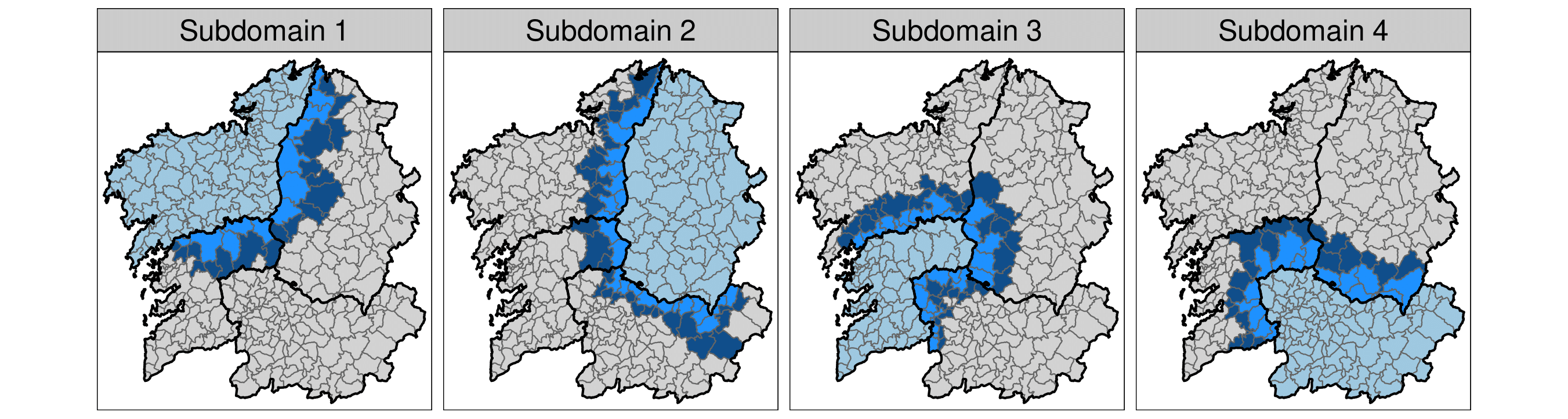
model="global", strategy="gaussian")When the number of small areas and time periods increases considerably (as is the case of analysing count data at municipality level), fitting the Global model becomes computationally very demanding or even unfeasible. Instead of considering global random effects whose correlation structures are based on the whole spatial/temporal neighbourhood graphs of the areal-time units, we propose to divide the data into \(D\) spatial subdomains. Doing so, local spatio-temporal models can be fitted simultaneously (in parallel or distributed) substantially reducing the computational time. In what follows, we show how to fit the Disjoint and k-order neighbourhood models (extending the methodology described in Orozco-Acosta et al. (2021)) for estimating spatio-temporal disease risks using the STCAR_INLA() function.
Disjoint model
Note that in the Disjoint model each area-time unit belongs to a single subdomain. Consequently, the log-risk surface \(\log{\boldsymbol{r}} = (\log{\boldsymbol{r}_1},\ldots,\log{\boldsymbol{r}_{D}})^{'}\) is just the union of the posterior marginal estimates of each spatio-temporal sub-model.
For our example data in Data_LungCancer we propose to divide the data into the \(D_s=47\) provinces of continental Spain. To classify the areas into provinces, the first two digits of the ID.area variable is used.
Carto_SpainMUN$ID.prov <- substr(Carto_SpainMUN$ID,1,2)In the code below, we show how to fit the Disjoint model with Type I space-time interaction random effect and Gaussian approximation strategy using 4 local clusters (in parallel)
Disjoint <- STCAR_INLA(carto=Carto_SpainMUN, data=Data_LungCancer,
                       ID.area="ID", ID.year="year", O="obs", E="exp", ID.group="ID.prov",
                       spatial="BYM2", temporal="rw1", interaction="TypeI",
                       model="partition", k=0, strategy="gaussian",
                       plan="cluster", workers=rep("localhost",4))
#> STEP 1: Pre-processing data
#> STEP 2: Fitting partition (k=0) model with INLA
#> + Model 1 of 47
#> + Model 2 of 47
#> ...
#> + Model 47 of 47
#> STEP 3: Merging the results

summary(Disjoint)
#> Time used:
#>     Running = 292, Merging = 377, Total = 669, NA = NA
#> Random effects:
#>   Name     Model
#>     ID.area BYM2 model
#>    ID.year RW1 model
#>    ID.area.year IID model
#>
#> Deviance Information Criterion (DIC) ...............: 339082.27
#> Deviance Information Criterion (DIC, saturated) ....: 148898.26
#> Effective number of parameters .....................: 3484.01
#>
#> Watanabe-Akaike information criterion (WAIC) ...: 339030.62
#> Effective number of parameters .................: 3275.68
#>
#>  is computed
#> Posterior summaries for the linear predictor and the fitted values are computed
#> (Posterior marginals needs also 'control.compute=list(return.marginals.predictor=TRUE)')
* Computations are made in personal computer with a 3.41 GHz Intel Core i5-7500 processor and 32GB RAM using R-INLA stable version INLA_25.06.07.
k-order neighbourhood model
Assuming independence between areas belonging to different sub-domains could be very restrictive and it may lead to border effects. The k-order neighbourhood model avoids this undesirable issue by adding neighbouring areas to each partition of the spatial domain.
Since multiple estimates of the linear predictor are obtained for some areal-time units from the different submodels, their posterior estimates must be properly combined to obtain a single posterior distribution for each \(\log{r_{it}}\). Two merging strategies could be considered here:
- If the
merge.strategy="mixture"argument is specified, mixture distributions of the estimated posterior probability density functions with weights proportional to the conditional predictive ordinates (CPO) are computed. See Orozco et al. (2021) for further details. - If the
merge.strategy="original"argument is specified (default option), the posterior marginal estimate of the areal-unit corresponding to the original submodel is selected.
In the code below, we show how to fit the 1st-order neighbourhood model with Type I space-time interaction random effect and Gaussian approximation strategy using 4 local clusters (in parallel)
options(future.globals.maxSize = 1.5*1e9) ## 1.5 GB

order1 <- STCAR_INLA(carto=Carto_SpainMUN, data=Data_LungCancer,
                     ID.area="ID", ID.year="year", O="obs", E="exp", ID.group="ID.prov",
                     spatial="BYM2", temporal="rw1", interaction="TypeI",
                     model="partition", k=1, strategy="gaussian",
                     plan="cluster", workers=rep("localhost",4))
#> STEP 1: Pre-processing data
#> STEP 2: Fitting partition (k=1) model with INLA
#> + Model 1 of 47
#> + Model 2 of 47
#> ...
#> + Model 47 of 47
#> STEP 3: Merging the results

summary(order1)
#> Time used:
#>     Running = 337, Merging = 1685, Total = 2022, NA = NA
#> Deviance Information Criterion (DIC) ...............: 339011.70
#> Deviance Information Criterion (DIC, saturated) ....: 148827.69
#> Effective number of parameters .....................: 3272.38
#>
#> Watanabe-Akaike information criterion (WAIC) ...: 338976.04
#> Effective number of parameters .................: 3092.34
#>
#>  is computed
#> Posterior summaries for the linear predictor and the fitted values are computed
#> (Posterior marginals needs also 'control.compute=list(return.marginals.predictor=TRUE)')
* Computations are made in personal computer with a 3.41 GHz Intel Core i5-7500 processor and 32GB RAM using R-INLA stable version INLA_25.06.07.
Plot the results
Once the model is fitted, maps of posterior median estimates of log-relative risks \(\log{r_{it}}\) and posterior exceedence probabilities \(P(\log{r_{it}}>0 | {\bf O})\) can be plotted using the tmap library as
library(tmap)
library(RColorBrewer)

tmap4 <- packageVersion("tmap") >= "3.99"

## Results for 1st-order neighbourhood model ##
Model <- order1

S <- length(unique(Data_LungCancer$ID))
T <- length(unique(Data_LungCancer$year))
t.from <- min(Data_LungCancer$year)
t.to <- max(Data_LungCancer$year)
## Maps of posterior median estimates of the linear predictor (log-risks) ##
log.risks <- matrix(Model$summary.linear.predictor$`0.5quant`, nrow=S, ncol=T, byrow=F)
colnames(log.risks) <- paste("Year", seq(t.from,t.to), sep=".")

carto <- cbind(Carto_SpainMUN,log.risks)

paleta <- brewer.pal(8,"RdYlGn")[8:1]
values <- c(0,0.67,0.77,0.83,1,1.20,1.30,1.50,Inf)

if(tmap4){
  Map.risks <- tm_shape(carto) +
    tm_polygons(fill=paste("Year",round(seq(t.from,t.to,length.out=9)),sep= "."),
                fill.scale=tm_scale(values=paleta, breaks=log(values), midpoint=0, interval.closure="left"),
                fill.legend=tm_legend("log-risks", show=TRUE, reverse=TRUE,
                                      position=tm_pos_out("right","center"),
                                      frame=FALSE),
                fill.free=FALSE, col_alpha=0) +
    tm_grid(n.x=5, n.y=5, alpha=0.2, labels.format=list(scientific=T),
            labels.inside.frame=F, labels.col="white") +
    tm_layout(panel.labels=as.character(round(seq(t.from,t.to,length.out=9))),
              panel.label.size=1.5) +
    tm_facets(nrow=3, ncol=3)
}else{
  Map.risks <- tm_shape(carto) +
    tm_polygons(col=paste("Year",round(seq(t.from,t.to,length.out=9)),sep= "."),
                palette=paleta, title="log-risks", legend.show=T, border.col="transparent",
                legend.reverse=T, style="fixed", breaks=log(values), midpoint=0, interval.closure="left") +
    tm_grid(n.x=5, n.y=5, alpha=0.2, labels.format=list(scientific=T),
            labels.inside.frame=F, labels.col="white") +
    tm_layout(main.title="", main.title.position="center", panel.label.size=1.5,
              legend.outside=T, legend.outside.position="right", legend.frame=F,
              legend.outside.size=0.2, outer.margins=c(0.02,0.01,0.02,0.01),
              panel.labels=as.character(round(seq(t.from,t.to,length.out=9)))) +
    tm_facets(nrow=3, ncol=3)
}
print(Map.risks)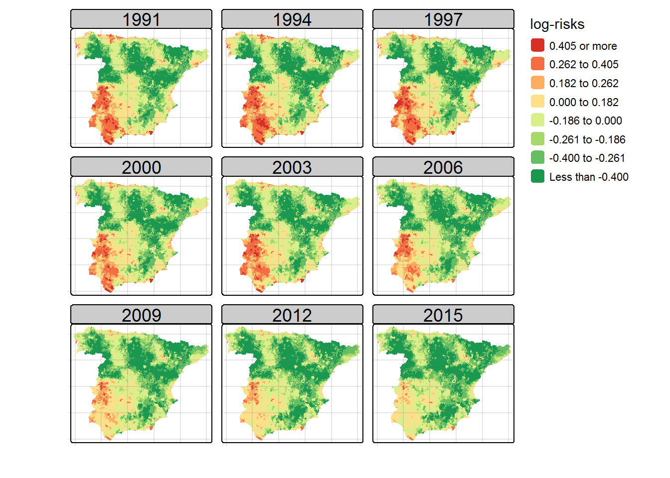
## Maps of posterior exceedence probabilities ##
probs <- matrix(1-Model$summary.linear.predictor$`0cdf`, nrow=S, ncol=T, byrow=F)
colnames(probs) <- paste("Year", seq(t.from,t.to), sep=".")

carto <- cbind(Carto_SpainMUN,probs)

paleta <- brewer.pal(6,"Blues")[-1]
values <- c(0,0.1,0.2,0.8,0.9,1)

if(tmap4){
  Map.probs <- tm_shape(carto) +
    tm_polygons(fill=paste("Year",round(seq(t.from,t.to,length.out=9)),sep= "."),
                fill.scale=tm_scale(values=paleta, breaks=values, interval.closure="left",
                                    labels=c("[0-0.1)","[0.1-0.2)","[0.2-0.8)","[0.8-0.9)","[0.9-1]")),
                fill.legend=tm_legend("", show=TRUE, reverse=TRUE, frame=FALSE,
                                      position=tm_pos_out("right","center")),
                fill.free=FALSE, col_alpha=0) +
    tm_grid(n.x=5, n.y=5, alpha=0.2, labels.format=list(scientific=T),
            labels.inside.frame=F, labels.col="white") +
    tm_layout(panel.labels=as.character(round(seq(t.from,t.to,length.out=9))),
              panel.label.size=1.5) +
    tm_facets(nrow=3, ncol=3)
}else{
  Map.probs <- tm_shape(carto) +
    tm_polygons(col=paste("Year",round(seq(t.from,t.to,length.out=9)),sep="."),
                palette=paleta, title="", legend.show=T, border.col="transparent",
                legend.reverse=T, style="fixed", breaks=values, interval.closure="left",
                labels=c("[0-0.1)","[0.1-0.2)","[0.2-0.8)","[0.8-0.9)","[0.9-1]")) +
    tm_grid(n.x=5, n.y=5, alpha=0.2, labels.format=list(scientific=T),
            labels.inside.frame=F, labels.col="white") +
    tm_layout(main.title="", main.title.position="center", panel.label.size=1.5,
              legend.outside=T, legend.outside.position="right", legend.frame=F,
              legend.outside.size=0.2, outer.margins=c(0.02,0.01,0.02,0.01),
              panel.labels=as.character(round(seq(t.from,t.to,length.out=9)))) +
    tm_facets(nrow=3, ncol=3)
}
print(Map.probs)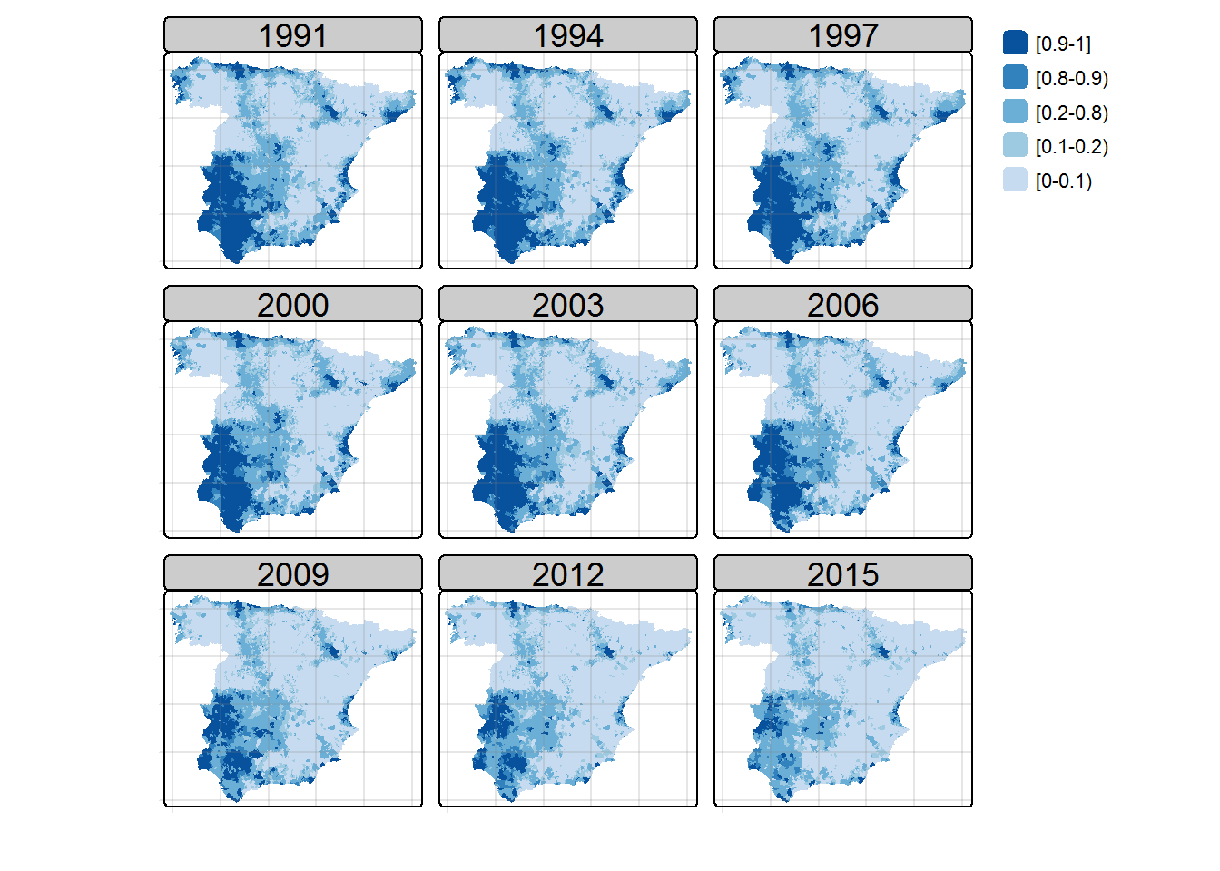
Acknowledgments
This work has been supported by Project MTM2017-82553-R (AEI/FEDER, UE) and Project PID2020-113125RB-I00/MCIN/AEI/10.13039/501100011033. It has also been partially funded by the Public University of Navarra (project PJUPNA2001).